

Recently, I have been doing a bit or research: given the recent advances in various AI disciplines, how practicable is it to use AI to predict bank customer behaviour based on peer group behaviour. To be more precise, the question was, which subcategory of AI lends itself the best for such prediction. And are such predictions good enough?

TL;DR: Neural Networks bear the palm, see at the bottom of the blog.
The evaluated AIs were
- Large Language Models (LLM), and within that text-embedding-ada-002 from OpenAi and BERT from Google
- Machine Learning (ML) via Support Vector Machines and Random Forest models
- Neural Networks via the Tensorflow Keras API
The data for the test were simple.They are anonymised data set of account balances from years of 2021 and 2022, stripped of all customer information except customer categories. The cohort was approx 20k customers, split into 16k training and 4k evaluation records.
Prediction of Giro to Tagesgeld shifts
To simplify the question of prediction, I was focusing on the following question: how much can we expect a customer to shift between her current account (Giro) and savings account (Tagesgeld TG). To normalise the data, we are not interested in the absolute amount, but in the percentage between -100% and +100%.
- 100% means all Giro funds are shifted to TG
- -100% means all TG is shifted onto Giro
- and 0 means not change
Large language models
Given the buzz of about generative AI the explosion of the quality of LLMs in particular, using language models was the first stop in the journey. The idea was to treat all the data we know on the customer as a text. Such text was then converted into a multi dimensional vector space via embeddings. The expectation is similar customers will point to similar “direction”
Embeddings in machine learning are representations of data, typically in a high-dimensional space, that capture the relationships and similarities between different data points. In the context of customer categorisation, embeddings translate customer segments, and other text data into numerical vectors that machine learning models can process.
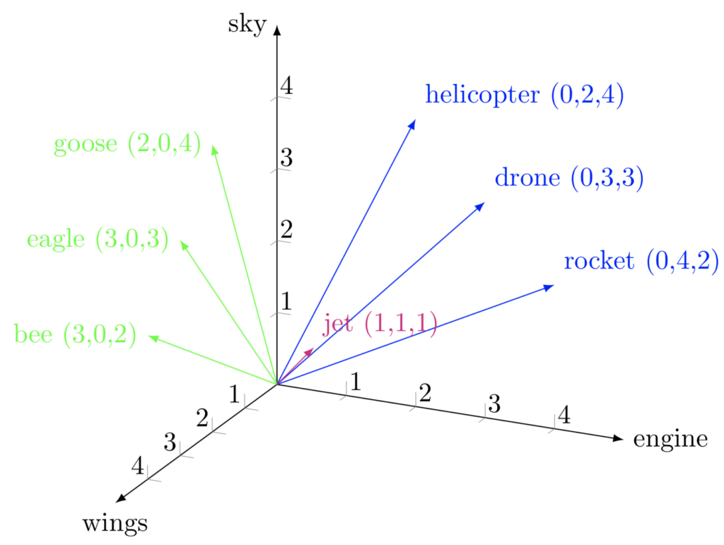
The above graphic depicts a simplified vector space of 3 dimensions, embedding the encodings of airborn objects. The embeddings of BERT tokens(words) will use a similar vector space with the dimensionality of 768. For OpenAI ADA the dimensions are as high as 1536.
Once your text data is converted into embeddings, we can feed this populated vector space into a machine learning model for the tasks of regression. This approach enables the model to make sense of the textual data and perform regression analysis based on the learned patterns and relationships in the embedded space. I have evaluated both The support vector machine used previously in my face recognition tool, and the more commonly used Random Forest model.
OpenAI Ada
class OpenAiAdaModel(ModelInterface):
    def __init__(self):
        logging.info(f"OpenAiAdaModel created")

    def initialize(self):
        logging.info(f"intialise OpenAI model")

        openai.api_key = self.api_key


    def embeddings(self, text: str) -> List[float]:

        response = openai.embeddings.create(input=text, model="text-embedding-ada-002")

        return response.data[0].embedding
While it is very easy to use the model of OpenAI, the combinations of remote call, and pay-per-call renders this approach unusable. Embeddings API calls take up to 500 miliseconds and USD 0.0001 per call, so we are looking at more than 2 hours of embedding run through time, with rather marginal costs of 2 USD. As various embeddings must be tested with different text representations, this is just not practical.
Enter Goggle BERT
Unlike the OpenAI embeddings, BERT can be run locally via the transformers package, which great improvement of speed. The BERT model will populate our vector space (conver the customer data to numbers) in few seconds.
from typing import List
from transformers import BertTokenizer, BertModel
import torch
import logging

from chupr.model.model import ModelInterface

class Bert(ModelInterface):
    def __init__(self):
        self.model = None
        self.tokenizer = None

    def initialize(self):
        self.tokenizer = BertTokenizer.from_pretrained('bert-base-uncased')
        self.model = BertModel.from_pretrained('bert-base-uncased')

    def embeddings(self, text: str) -> List[float]:
        logging.debug(f"Embeddings for {text}")
        inputs = self.tokenizer(text, return_tensors="pt")
        with torch.no_grad():
            outputs = self.model(**inputs)
        return outputs.last_hidden_state[:, 0, :][0].tolist()
Unfortunately, the trained Random Forest regression fitted over this vector space is very noisy. The mean average error within the same year is 20%, and it raises to 50% when prediction is attempted year over year, basically useless. One possible explanation is that textual similarities in our data representation are not well suited for LLM, which has been trained on unstructured text data.
As embedding did not yield, we must try other means to prepare our data for ML fitting.
One-Hot encoding
Embeddings above were used to turn the text categories of customers to numeric representation. Fortunately, the toolbox of data science provides a different standard solution for this problem: one-hot encoding.
One-hot encoding in machine learning transforms categorical text data into numerical format. It involves creating binary vectors for each category, where each vector’s length equals the number of unique categories. In these vectors, 1 represents the presence of the category, and 0s indicate absence. This method ensures clear distinction between categories and is straightforward to implement. One-hot encoding doesn’t capture relationships between categories, making it most suitable for datasets with limited unique categories, which is our case for the approx 10 categories we place our customers into.
Python pandas, as always, have a tool in its toolbelt to achieve this with
df_features_encoded = pd.get_dummies(df_features, columns=text_features)The resulting regression is now more stable. The following chart represents the 2021 training data in blue and the test data in orange
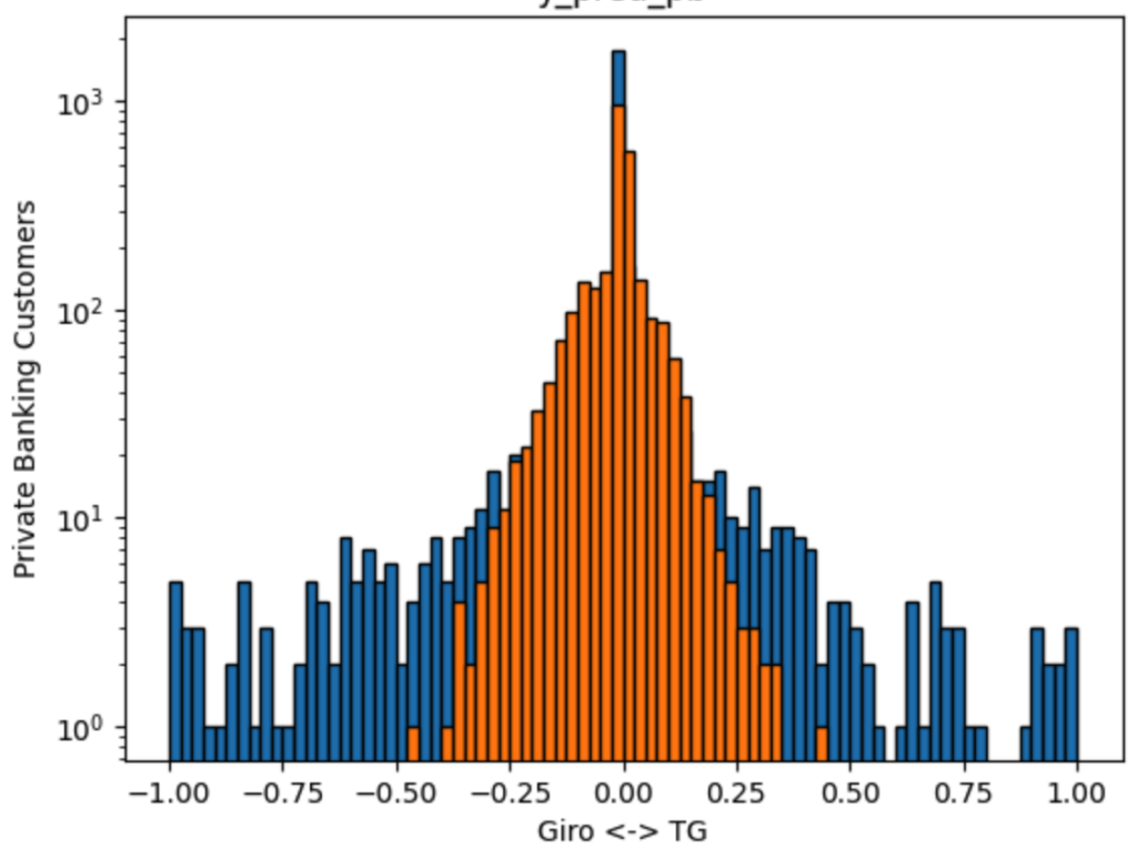
Two things can be noticed here:
- The majority of the customers dont shift funds (most of the data are around 0%)
- There is too little data on the tails to fit this regressor.
The prediction quality improves nevertheless. We have now a mean average error of 8% within the same year, and 20% year on year.
Testing with other ML regressors and other model parameters from the scikit learn toolbox shows no significant improvement over this 8% / 20% error. We need to try something different: neural networks.
Neural Networks Prediction
Here, we will be keeping the one-hot encoding introduced above, and replacing the ML regressors with Deep Neural Network. This can be done with minimal changes to our code, thanks to the excellent Keras Tensorflow API.
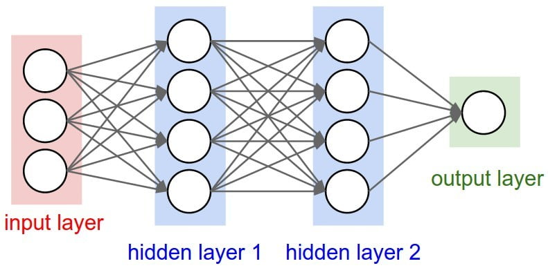
Deep Neural Networks (DNNs) are advanced machine learning models inspired by the human brain’s structure and function. They consist of multiple layers of interconnected nodes or “neurons,” with each layer performing complex transformations on data. These layers include input, hidden, and output layers. Hidden layers, where most data processing occurs, allow DNNs to learn and model intricate patterns and relationships in large datasets. Their “deep” architecture enables them to capture subtle nuances, but they require substantial data and computational power to train effectively. Our DNN with have a depth of merely 2 hidden layers of 1024 neurons.
Neural networks typically perform better on normalized data. One additional thing we must do with our data therefore is to normalise them for the DNN processing.
X_train, X_test, y_train, y_test = train_test_split(X, y, test_size=0.2, random_state=42)

scaler = StandardScaler()
X_train = scaler.fit_transform(X_train)
X_test = scaler.transform(X_test)
The setup of the DNN via Keras is very simple. We define the input layer to pick up our train data dataframe, two hidden layers, and an output layer.
neuron_count = 1024
model = Sequential([
    Dense(neuron_count, activation='relu', input_shape=(X_train.shape[1],)),
    Dense(neuron_count, activation='relu'),
    Dense(neuron_count, activation='relu'),
    Dense(1)  # Output layer
])
model.compile(optimizer='adam', loss='mean_squared_error', metrics=['mae'])
history = model.fit(X_train, y_train, epochs=400, batch_size=32)
Lets go into the details here. The choice of relu as activation function and adam as optimiser are rather typical configs, and have not been evaluated further. The 1024 neuron wide layer provided only marginal benefit over the 512 wide. Batch size of 32 was shown to perform better than 16 or 64.
The explanation for the rather large epoch count is that the model tends to converge rather slowly (mean squared error/epochs):

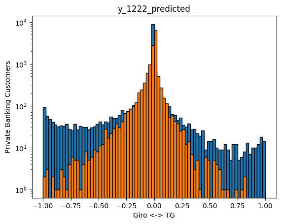
Such 400 iterations take approx 30 minutes on a Intel Core i7-8850H CPU, keeping in mind the single threaded nature or Python interpreter. It can be argued, that the precision could be increased at the cost of more CPU power/time, as the above curve has not flattened out yet. Nevertheless, we reach 4% mean average error within the year, with 11% year on year. More importantly, the predictions (in orange) now also capture the tails much better. The resulting DNN has 2 mio weights.
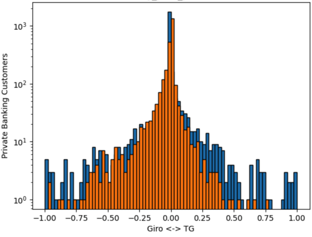
Predictions for 2022 exhibit something else interesting. While our predictions (orange) cover the tails to the similar extent as our training data for 2021, the real 2022 data have much fatter tails. The shape of the 2022 distribution is much less centered on 0% now. It can be speculated, that this is the effect of customer reactions to higher interest rates, not existent in the zero intrest rate environment of 2021, hence not trainable on 2021 data.
Summary: What is good enough prediction
Lets recap what we have: we have a model, that predicts the behaviour of customers within the year to the precision of 96%. For the next year, this decreases to 88%, most likely due to interest rate changes. Albeit the precision is still good around the mean, it gradually degrades when more than 10% funds are shifted between Giro and TG.
Such predictions are certainly very useful both within the same year, and also year over year, if bulk behaviour of customers are of interest, eg for treasury. The good precision of the model within the same year even makes it valuable for marketing or customer communication, as customer actions can be anticipated with the precision of 96% over short term periods.